Hello, this is MiTornAve.
In our 2-2 session, we explored the 'memory' of RNN and LSTM, which understand context by remembering the flow of time. It was fascinating to see how AI mimics human thought processes by not forgetting past information to predict the future.
However, in actual industrial sites or high-level engineering design fields, 'overwhelming processing speed' is often as vital as 'accurate memory.' For instance, consider situations where sensor data changing every few milliseconds (ms) must be calibrated in real-time, or the output of a complex system needs to be predicted instantaneously.
The model we are introducing today, the RBFNN (Radial Basis Function Neural Network), stands at the pinnacle of such 'speed' and 'efficiency.' Let’s dive into the identity of this model, a regular fixture in control systems and numerical prediction papers.
1. Global Learning vs. Local Response: The Philosophy of RBFNN
The Multi-Layer Perceptron (MLP) we commonly know is a system where all neurons are interconnected, and the weights of the entire network are slightly modified every time data enters. This is called 'Global Learning.' However, a disadvantage is that learning speed slows down as data volume increases.
RBFNN takes a completely different approach by focusing on 'Local Response.' Let’s analyze the specific differences and philosophy in detail.
1.1 Global Learning (MLP): "A Massive System Where Everyone Changes Slightly"
Operating Principle: In an MLP, a single piece of input data affects all layers and all weights (W) within the network. The entire network reacts every time data is input.
Inefficiency: Since all neurons are activated to adjust the entire weight set to reduce error, the computational load increases exponentially as data becomes vast.
The Trap of Long-Term Memory: When learning new data, previously established weights can be disrupted globally. This often leads to stagnated learning speeds or the loss of previously learned information.
1.2 Local Response (RBFNN): "An Efficient System Where Only Necessary Parts Wake Up"
RBFNN divides the input space into several 'regions' and activates only the neurons responsible for the specific region where the input value falls.
Economies of Scope (Radial Basis):
Instead of scanning the entire dataset, it measures how close the input value is to a specific region's Center.
As it moves away from the center (c_i), the responsiveness drops sharply, and it only produces a meaningful output when within a certain Radial distance. In other words, it does not respond to irrelevant data at all.
Radar System (Local Approximation):
It is similar to installing multiple radars on a map; a specific radar reacts strongly only when an object enters its line of sight.
Each hidden layer neuron has its own 'defense range.' If the input data is not in its designated area, it remains inactive and only precisely analyzes data that enters its zone.
1.3 Why is RBFNN 'Ultra-Fast'?
This 'Local Response' philosophy creates an overwhelming difference in actual learning and inference speeds.
Computational Optimization: Unlike MLP, there is no need to update tens of thousands of weights simultaneously. Only the neurons located near the current input value participate in the calculation.
Independent Learning: Since each neuron is responsible for a specific area, learning in one region does not interfere with information in other regions, resulting in very fast convergence.
Mathematical Simplicity: After calculating the distance via a Gaussian function in the hidden layer, the output layer simply performs a Linear Sum. This allows for the optimal solution to be derived instantly using linear algebraic techniques without complex repetitive iterations.
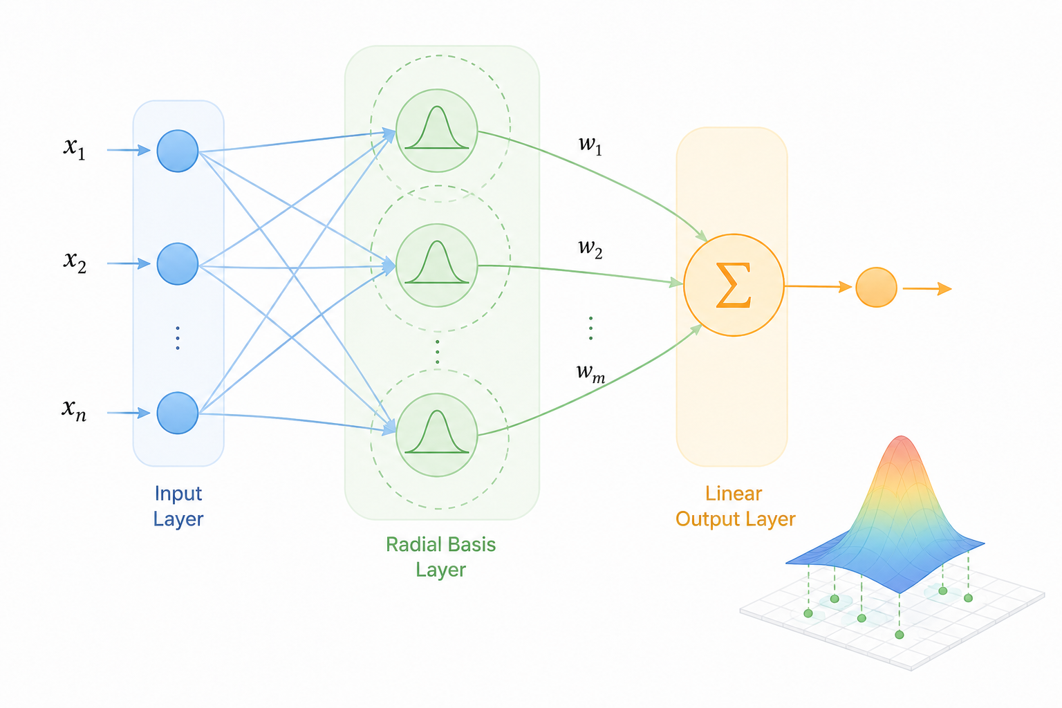
2. The Structure of RBFNN: The Aesthetics of Speed Created by Simplicity
RBFNN differs from deep learning models that stack complex multiple layers. It solves everything with just three layers, using a horizontal structure to dramatically reduce computational complexity while maintaining strong approximation capabilities.
Input Layer: The gateway for external data. It passes the input values directly to the hidden layer without any calculation.
Hidden Layer: The core section where the 'intelligence' of the RBFNN is determined. Instead of the usual weighted sums, each neuron uses a Gaussian Function to calculate the distance between the input and its Center. The closer the input is to the center, the closer the output value is to 1.
Output Layer: Produces the final result by multiplying the local response values from the hidden layer by weights. This step consists of a simple Linear Sum, effectively concluding by treating a non-linear problem as a linear one.
2.1 Why is it so Fast? (Separation of Learning)
RBFNN is hailed as an 'ultra-fast model' because the learning process is structurally dualized.
Unsupervised Learning Phase (Hidden Layer): First, data distribution is analyzed to place centers for the hidden layer neurons. Clustering techniques like FCM (Fuzzy C-Means) or K-Means are typically used.
Supervised Learning Phase (Output Layer): Once the centers are fixed, the remaining task is simply determining the weights of the output layer. This does not require tens of thousands of backpropagation iterations; instead, the mathematically optimal solution can be calculated in one-shot using the Least Squares Method.
2.2 RBFNN vs. MLP: How Structural Differences Direct Performance
The two models differ significantly in how they perceive data:
Structural Difference: MLP takes a vertical form with multiple hidden layers, whereas RBFNN has a wide, horizontal structure with a single hidden layer.
Neuron Mechanism: MLP uses non-linear activation functions like Sigmoid, while RBFNN uses distance-based Gaussian functions.
Learning Scope: MLP follows a global learning approach where all neurons participate simultaneously, but RBFNN uses a local approach where only neurons in a specific area react.
Learning Speed: MLP is relatively slow due to repeated backpropagation. RBFNN is very fast because it separates the learning process and uses linear operations at the output.
Application: MLP is suitable for deep reasoning like image recognition, while RBFNN excels in real-time control, time-series prediction, and precise function approximation.
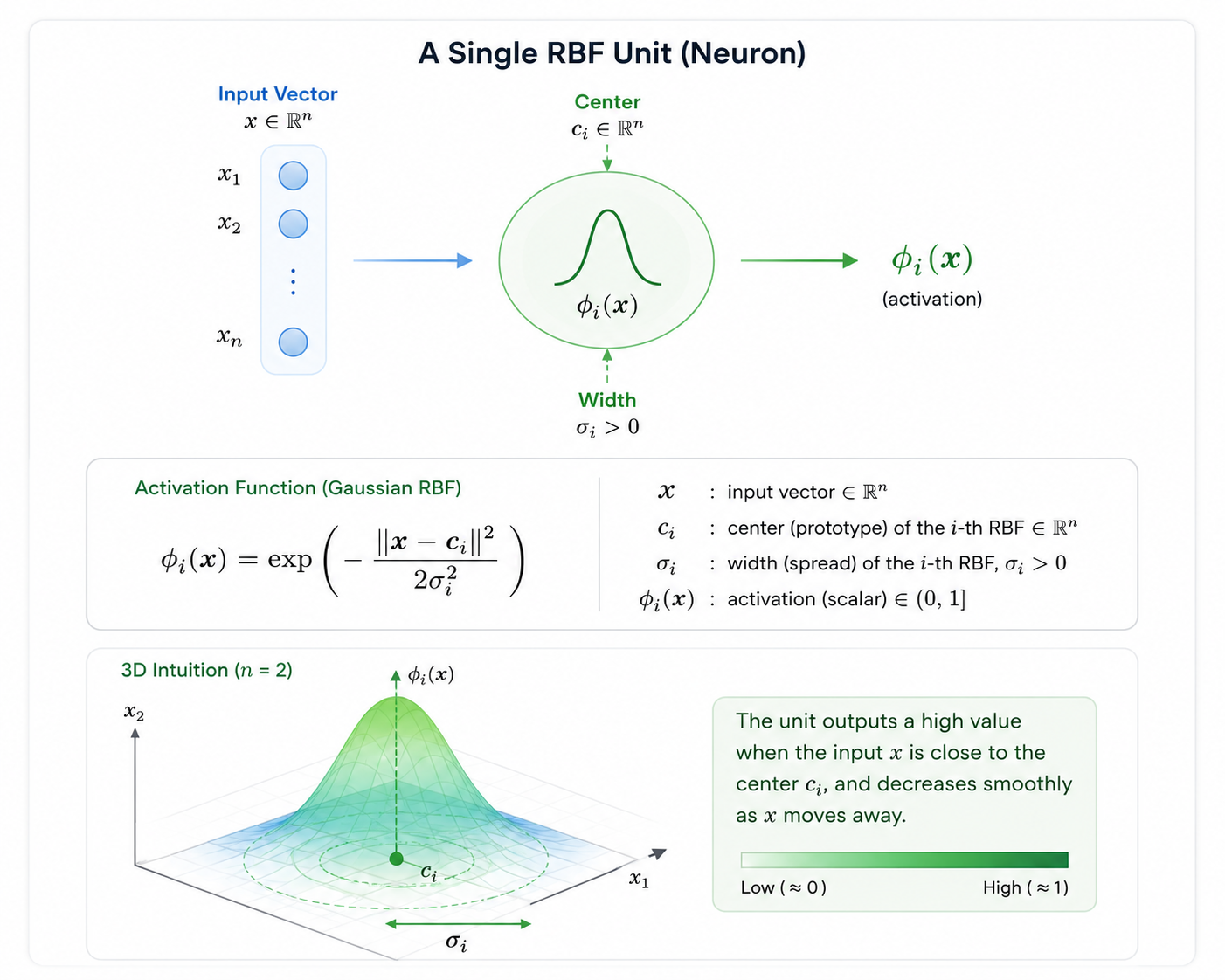
3. Anatomy of the Equation: Intelligence Judged by Distance
The magic happening in the RBFNN hidden layer is summarized by the following equation:
\phi(x) = \exp\left(-\frac{\|x - c_i\|^2}{2\sigma_i^2}\right)
\|x - c_i\|: The distance between the input (x) and the center (c_i). The closer the distance, the closer the result is to 1; the further away, the more it converges to 0.
\sigma (Sigma): The width of the responding range. A large value covers a wide area, while a small value makes the neuron sensitive to a very narrow region.
4. RBFNN vs. MLP: When to Use Which?
If you are torn between the two models for a paper or project, consider these criteria:
4.1 Comparison of Key Features
Learning Speed: MLP is slow (requires iterative learning), whereas RBFNN is very fast (primarily linear operations).
Structural Flexibility: MLP allows for deep, multi-layer structures. RBFNN is basically a single-hidden-layer structure.
Data Approximation: MLP focuses on global features, while RBFNN specializes in local regions.
4.2 Selection Guide by Situation
Image Recognition and Complex Classification: MLP is better suited for extracting abstract features from high-dimensional data.
Real-time System Control: RBFNN is advantageous for processing data changing every second where computational resources are limited.
Time-series Prediction and Function Approximation: RBFNN shows superior efficiency in engineering problems requiring precise numerical range predictions.
[Practice Section] Verifying the Local Response of RBFNN
The core principle is: Close to center \rightarrow Strong activation / Far from center \rightarrow Rapid drop to 0.
Python Version
Python
# ============================================================
# Radial Basis Function Neural Network (RBFNN) - Basic Example
# Gaussian RBF Activation Visualization
# ============================================================

import numpy as np
import matplotlib.pyplot as plt

# ------------------------------------------------------------
# Gaussian Radial Basis Function
# φ(x) = exp( -||x - c||² / (2σ²) )
#
# x      : input
# c      : center of the neuron
# sigma  : width (spread) of the Gaussian
# ------------------------------------------------------------
def gaussian_rbf(x, center, sigma):
    distance_squared = np.linalg.norm(x - center) ** 2
    return np.exp(-distance_squared / (2 * sigma ** 2))


# ------------------------------------------------------------
# Hyperparameters
# ------------------------------------------------------------
center = 0.0
sigma = 1.0

# Input range
x_values = np.linspace(-5, 5, 200)

# Compute RBF outputs
rbf_outputs = []

for x in x_values:
    y = gaussian_rbf(x, center, sigma)
    rbf_outputs.append(y)

rbf_outputs = np.array(rbf_outputs)


# ------------------------------------------------------------
# Print Example Outputs
# ------------------------------------------------------------
print("=== Gaussian RBF Outputs ===\n")

test_points = [0, 1, 2, 5]

for point in test_points:
    output = gaussian_rbf(point, center, sigma)

    print(f"Input x = {point}")
    print(f"RBF Output = {output:.6f}")

    if output > 0.7:
        print("→ Strong activation (input is close to the center)\n")

    elif output > 0.1:
        print("→ Moderate activation\n")

    else:
        print("→ Very weak activation (far from the center)\n")


# ------------------------------------------------------------
# Visualization
# ------------------------------------------------------------
plt.figure(figsize=(10, 5))

plt.plot(
    x_values,
    rbf_outputs,
    linewidth=3,
    label='Gaussian RBF'
)

# Mark center point
plt.scatter(
    [center],
    [gaussian_rbf(center, center, sigma)],
    s=100,
    label='Center'
)

plt.title("Gaussian Radial Basis Function", fontsize=16)
plt.xlabel("Input x", fontsize=12)
plt.ylabel("Activation φ(x)", fontsize=12)

plt.grid(True, alpha=0.3)
plt.legend()

plt.show()
This demonstrates that when the input passes through the center (0), an output of 1 appears immediately, and as the input value moves further from the center, the output gradually decreases. (While the specific output values may vary depending on each individual RBFNN model, you can clearly observe that the output drops significantly when comparing inputs of 0, 1, and 5).
In fact, rather than being a general-purpose tool, the RBFNN model is extensively used across various engineering fields, including time-series analysis; therefore, many of you reading this are likely engineering students or professionals. (If not, that’s fine too!). Consequently, you will likely encounter this more often in MATLAB—the pride and soul of us engineers. Since I actually wrote my thesis based on this very code, I am leaving a MATLAB version here as well.
MATLAB Version
Matlab
% ============================================================
% Radial Basis Function Neural Network (RBFNN) Example
% Gaussian RBF Activation Function
% ============================================================

clc;
clear;
close all;

% ------------------------------------------------------------
% Parameters
% ------------------------------------------------------------
center = 0;
sigma = 1;

% Input range
x_values = linspace(-5, 5, 200);

% ------------------------------------------------------------
% Gaussian RBF Function
% φ(x) = exp(-(x-c)^2 / (2*sigma^2))
% ------------------------------------------------------------
rbf_outputs = exp(-((x_values - center).^2) ./ (2 * sigma^2));

% ------------------------------------------------------------
% Display Example Values
% ------------------------------------------------------------
fprintf('=== Gaussian RBF Outputs ===\n\n');

test_points = [0 1 2 5];

for i = 1:length(test_points)

    x = test_points(i);

    output = exp(-((x - center)^2) / (2 * sigma^2));

    fprintf('Input x = %.1f\n', x);
    fprintf('RBF Output = %.6f\n', output);

    if output > 0.7
        fprintf('-> Strong activation (close to center)\n\n');

    elseif output > 0.1
        fprintf('-> Moderate activation\n\n');

    else
        fprintf('-> Very weak activation (far from center)\n\n');
    end
end

% ------------------------------------------------------------
% Visualization
% ------------------------------------------------------------
figure('Color', 'w');

plot(x_values, rbf_outputs, 'LineWidth', 3);

hold on;

scatter(center, 1, 100, 'filled');

title('Gaussian Radial Basis Function');
xlabel('Input x');
ylabel('\phi(x)');

grid on;
5. Conclusion: A Powerful Tool for Practical Engineering
Today, we explored the RBFNN, which performs ultra-fast calculations using the intuitive concepts of 'distance' and 'range.' While current trends favor Deep Layers, RBFNN remains irreplaceable in fields where real-time performance is paramount.
With this, we have covered the primary weapons of AI: Vision (CNN), Memory (RNN/LSTM), and Speed (RBFNN).