Hello, this is MiTornAve.
In our 4th session, we explored how artificial intelligence gained the "eyes" of CNNs (Convolutional Neural Networks), which grasp the entanglement of 2D space and achieve visual abstraction. CNNs have surprised the world with their overwhelming performance in interpreting images.
However, not all data in the world exists like a single frozen photograph. Just as light implies the flow of time, AI had to understand the "axis of time" to possess true intelligence. For instance, a single image can tell us whether an animal is a cat or a dog.
But imagine we are building a control system for a self-driving car. If we equip a car with numerous sensors, can it drive itself based on a single piece of data captured right before departure? Of course not. In other words, a "memory device" is required so that the artificial neural network can operate in response to continuous changes within a dynamic system.
Today, we will move beyond a static view and delve into RNNs and LSTMs—the memory devices of AI that project yesterday's memories into today.
1. From Frozen Photos to Flowing Time: The Essence of Time-Series Data
Stock charts, weather changes, heartbeat graphs, and even the "sentences" we are sharing now—what do they have in common? It is that the "Sequence" of data has a decisive impact on the result.
"I had a delicious [ ? ] for lunch today."
To infer the word for this blank, you must remember the context of the previous words like "lunch" and "delicious". The Multi-Layer Perceptrons (MLP) or CNNs we learned about previously are like goldfish that cannot remember past data at all.
They are geniuses at interpreting hundreds of photos in a second, but they are completely hopeless at reading a novel page by page to understand the plot. These models treat every moment of incoming data as a completely new, independent event, entirely severed from the previous situation. It's like asking them to predict tomorrow's weather by looking only at the current thermometer reading, while completely forgetting that it rained yesterday and that dark clouds are gathering today.
Asking a model that has forgotten the past to predict the future was truly absurd. To move closer to "true intelligence" beyond the frozen moments, AI absolutely had to acquire the continuity of "memory" that connects yesterday's events to today.
2. RNN (Recurrent Neural Network): A Mathematical Loop Projecting the Past into the Present
To remember past information, scientists introduced a very intuitive yet groundbreaking structure into neural networks. They twisted the existing "Feed-forward" structure—where information only traveled straight from input to output—to create a "recurrent loop" where part of the output returns as input. This is the birth of the RNN (Recurrent Neural Network).
2.1 Hidden State (H_t): The 'Short-term Memory' Gained by Neural Networks
The greatest invention of the RNN is the Hidden State (H_t). This acts as a "memory storage" flowing within the neural network.
Overlap of Memory: An RNN does not judge based solely on the input value (X_t) at the current time (t). It determines the current state by blending it with H_{t-1}, the "summary of the past" calculated and passed down from the immediately preceding time step (t-1).
Recursive Structure: This process exactly matches how we keep the previous context in our minds to understand the meaning of the word we are currently reading in a novel. It is a method of "stacking time" rather than just stacking layers.
2.2 Anatomy of the Equation: Yesterday's Me and Today's Stimulus
The core equation determining the behavior of an RNN is simple but contains a powerful philosophy:
H_t = \tanh(W_{hh}H_{t-1} + W_{xh}X_t + b)
Meeting of Two Worlds: In the formula, the past (H_{t-1}) and the present (X_t) pass through their respective filters called weights (W) and merge into a single vector.
Fixed Weights: The key here is that the values of W_{hh} and W_{xh} do not change as time flows. In other words, the past and present are combined using the same "rule" at any point in time.
Stepping Stone to Tomorrow: The H_t calculated this way becomes the current output, but it is simultaneously passed as input to the next time step (t+1). The phrase "Yesterday's me (H_{t-1}) meets today's stimulus (X_t) to form a new me (H_t) to be passed to tomorrow" is not just a metaphor; it is the definition of the equation itself. (In reality, we often pass everything off to "Tomorrow's Me.")
2.3 Unrolling Through Time: The Giant Network Hidden Behind the Loop
While it may look like a single neuron spinning in a circle, the true power of an RNN is revealed when it is unrolled according to the sequence of time. If there are 5 inputs, it takes the form of 5 layers sharing the same weights connected horizontally. Consequently, an RNN becomes a "very deep neural network" that can lengthen flexibly depending on the data. This allows RNNs to respond flexibly to everything from very short words to long sentences.
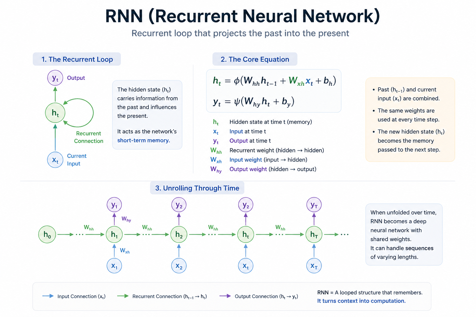
2.4 One-Line Summary: The Essence of RNN
Ultimately, an RNN is a model that turns "Context" into numbers. It has gained the "wisdom" to interpret the same input value completely differently depending on what it saw in the previous step. However, even in this beautiful recurrent structure, a "fatal weakness" was hidden: if the sequence becomes too long, it forgets the past.
3. Short-term Amnesia: The Long-Term Dependency Problem
Behind the mathematical elegance of RNNs lay a very realistic and painful limitation called the "Long-Term Dependency" problem. Understanding this problem is a crucial key to knowing why we had to move beyond simply stacking layers to complex structures like LSTM.
Ironically, although RNNs were born to remember time, they suffered from a fatal "forgetfulness". This is a phenomenon where the model completely forgets important information from the beginning of a sentence as the sentence gets even slightly longer.
3.1 "Came from France but can't speak French?"
Let's give the model an example that we humans can easily solve:
"I was born in France and lived there for 10 years. After that, I moved to Korea, went to school, got a job, blah blah blah... So, I am fluent in [ ? ]."
As humans, we instinctively know the answer is 'French' because we still keep the information about 'France' from the distant past in our heads. However, for a pure RNN, this problem is like an impregnable fortress. As information is passed back, the core keyword 'France' input at the beginning becomes increasingly diluted, until by the time it reaches the end, not even its shape remains.
3.2 Error Signals Blocked by the Wall of Time: Vanishing Gradient
Why does this happen? The culprit is the Vanishing Gradient problem we covered in Part 4.
The Pain of Going Back in Time: Training an RNN uses BPTT (Backpropagation Through Time), where errors travel back through time.
The Trap of the Chain Rule: To climb far back into the past, you must repeatedly multiply the derivative values of activation functions like Sigmoid or Tanh.
Convergence to Zero: If these derivative values are less than 1 (usually 0.25 or less), the error signal decreases exponentially through dozens of multiplications and eventually converges to 0.
3.3 No Tomorrow for a Model that Forgot the Past
Eventually, the weights close to the input layer—the very old ones—receive no signal telling them "how to update". Since old information disappears, the model becomes obsessed only with the last few words and misses the grand flow that penetrates the context. Although it's named 'Recurrent Neural Network,' it effectively becomes a halfway model that can barely maintain 'very brief short-term memory'.
To rescue these 'signals lost in the abyss,' engineers began to devise special devices that don't just overwrite memory but selectively store only important information. That is the true protagonist of Part 5, LSTM.
4. LSTM (Long Short-Term Memory): The Conveyor Belt Controlling Memory
In 1997, Sepp Hochreiter and others published the LSTM (Long Short-Term Memory) structure to cure the fatal forgetfulness of RNNs. The name itself is quite extraordinary, right? It contains the determination to take 'Short-Term Memory' and make it very 'Long.' This structure has served as the global standard for modern time-series data processing for decades.
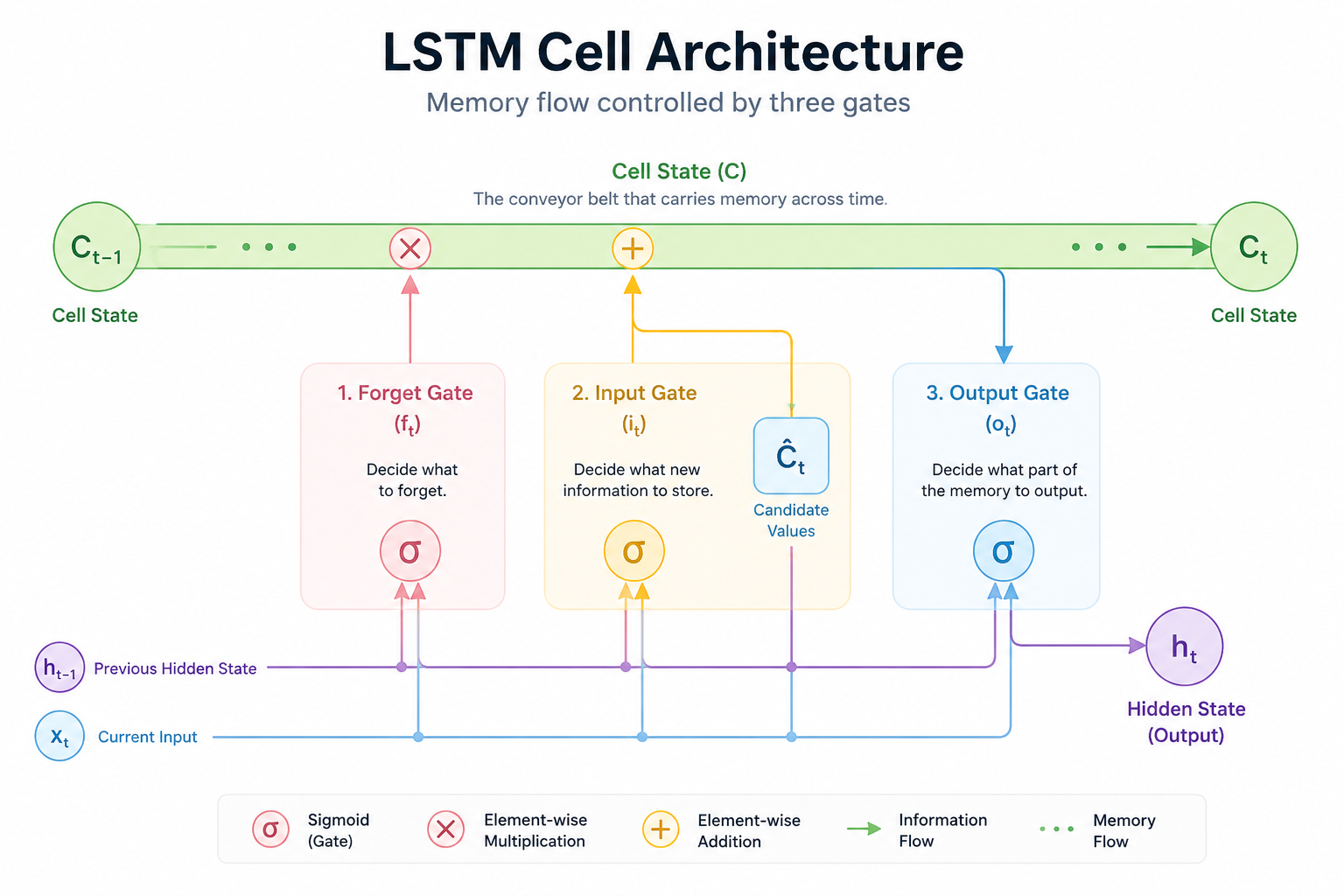
The genius of LSTM lies in the fact that, instead of recklessly cramming memory into the next step, it cleared a "highway" for information to flow and installed three sophisticated "Gates (Valves)" along that path.
4.1 Cell State (C_t): The Main Conveyor Belt Carrying Information
The heart of LSTM is the Cell State (C_t), which flows across the entire network.
Preservation of Information: This is like the main conveyor belt of a factory. Unlike an RNN, where information is transformed through complex calculations every time, LSTM places information on the belt and carries it to the end while only slightly adding or removing what is necessary.
The Key to Long-Term Memory: By securing a passage where information can flow intact without being lost midway, AI has finally gained the "long-term memory" to take a word from the very beginning of a sentence and not forget it until the end.
4.2 Three Gates: Smart Valves Managing Memory
To manage the memory flowing on the conveyor belt, LSTM utilizes three control devices. They decide how much to open or close the door with a value between 0 (completely blocked) and 1 (completely passed).
Forget Gate (f_t) - "What to discard?"
Decides 'how much to erase' from the past memory that is no longer needed.
For example, if the protagonist in a novel changes from 'Male' to 'Female,' the memory of 'Masculine Pronouns' maintained until then is boldly thrown off the belt.
Input Gate (i_t) - "What to add?"
Judges 'how much value there is to store' among the new information that has come in at the current moment.
Important keywords are newly placed on the belt, while trivial modifiers are just let go. In this process, the selected information finally joins the long-term memory (Cell State).
Output Gate (o_t) - "What to show?"
Based on the refined long-term memory (C_t), it calculates the final output (H_t) to be sent out at the current moment.
It doesn't just hold the memory; it acts as a filter to select and output the most appropriate 'answer' according to the current situation.
4.3 Summary: Why did LSTM win?
While RNNs collapsed from overload while trying to remember every bit of incoming information, LSTM learns for itself "what to forget, what to store, and what to output." Thanks to this, we now have amazing translators and voice assistants that can grasp context thousands of words away.
[Practice Section] Checking RNN's Memory in Google Colab
It’s time to check the mathematical principles directly through code. The following code is a very simple experiment using PyTorch to show how an RNN remembers and processes the flow of the word "hello."
Copy and execute (Shift + Enter) it in a blank cell.
Python
import torch
import torch.nn as nn
import torch.optim as optim
import numpy as np

# 1. Data Preparation
# Goal: Predict the next character ('h' -> 'e', 'e' -> 'l', 'l' -> 'l', 'l' -> 'o')
char_set = ['h', 'e', 'l', 'o']
input_size = len(char_set)  # 4 (One-hot size)
hidden_size = 8             # Dimensionality of memory
learning_rate = 0.1

# Mapping characters to indices and vice versa
char_to_idx = {c: i for i, c in enumerate(char_set)}
idx_to_char = {i: c for i, c in enumerate(char_set)}

# Input: 'hell', Target: 'ello'
x_data = [char_to_idx[c] for c in 'hell']
y_data = [char_to_idx[c] for c in 'ello']

# Convert to One-hot Encoding
# Shape: (Sequence_length, Batch_size, Input_size) -> (4, 1, 4)
x_one_hot = [np.eye(input_size)[x] for x in x_data]
X = torch.FloatTensor(x_one_hot).unsqueeze(1)
Y = torch.LongTensor(y_data)

# 2. Define Model
class SimpleRNN(nn.Module):
    def __init__(self, input_dim, hidden_dim, output_dim):
        super(SimpleRNN, self).__init__()
        self.rnn = nn.RNN(input_dim, hidden_dim, batch_first=False)
        self.fc = nn.Linear(hidden_dim, output_dim) # Decode memory to character prediction

    def forward(self, x, hidden):
        out, h_n = self.rnn(x, hidden)
        # Reshape output to pass through Linear layer
        # out shape: (Seq, Batch, Hidden) -> (4, 1, 8)
        out = self.fc(out.view(-1, hidden_dim))
        return out, h_n

model = SimpleRNN(input_size, hidden_size, input_size)

# 3. Loss & Optimizer
criterion = nn.CrossEntropyLoss()
optimizer = optim.Adam(model.parameters(), lr=learning_rate)

# 4. Training Loop
print("--- Training Started ---")
for epoch in range(100):
    model.train()
    optimizer.zero_grad()

    # Initialize hidden state (Batch_size=1, Layers=1, Hidden_dim=8)
    hidden = torch.zeros(1, 1, hidden_size)

    # Forward pass
    outputs, _ = model(X, hidden)

    # Calculate loss
    loss = criterion(outputs, Y)

    # Backward and optimize
    loss.backward()
    optimizer.step()

    # Check intermediate results
    if (epoch + 1) % 20 == 0:
        result = outputs.data.numpy().argmax(axis=1)
        result_str = ''.join([idx_to_char[c] for c in result])
        print(f"Epoch [{epoch+1}/100], Loss: {loss.item():.4f}, Predict: {result_str}")

# 5. Final Result Check
print("\n--- Final Prediction Result ---")
model.eval()
with torch.no_grad():
    hidden = torch.zeros(1, 1, hidden_size)
    outputs, _ = model(X, hidden)
    final_idx = outputs.data.numpy().argmax(axis=1)
    final_str = ''.join([idx_to_char[c] for c in final_idx])
    print(f"Input: 'hell' -> Predicted: '{final_str}'")
By running this code, you can see how data is processed through 5 time steps (Sequence) and how the final "Hidden State," which compresses the preceding information, is structured at the last moment.
The Python code may look a bit complex, but the core is "training the AI to see the letters 'hell' and answer 'ello'." Let's find out what happens at each step.
What do you input and what do you expect? (Input & Target)
Vocabulary: We use only 4 letters: h, e, l, o.
Input: We input h -> e -> l -> l (hell) one by one in order.
Target: The model should answer e -> l -> l -> o (ello).
In other words, it is a process of learning to answer 'e' when it sees 'h', and 'l' when it sees 'e'.
Conversion into a computer-understandable format (Encoding)
Since computers cannot read letters directly, they must be changed into numbers.
One-hot Encoding: Since there are 4 types of letters, each letter is made into a 4-dimensional list. For example, h = [1, 0, 0, 0], e = [0, 1, 0, 0]... It’s a method where only 'my position' is marked with a 1.
Structure of the Model (SimpleRNN Class)
This model is roughly divided into two parts:
RNN Layer: It looks at the incoming letters and updates its memory (Hidden State), thinking, "These letters have come in so far."
Linear Layer (FC): Based on the 'memory' created by the RNN, it makes a final judgment, saying, "So the probability that the next letter is 'e' is 80%."
Usage and Training Process (Training Loop)
When you run the code, training proceeds in the following order:
Memory Initialization: Since it hasn't seen anything at first, it fills the memory (hidden) with 0 and starts.
Prediction: Show 'hell' to the model and listen to its answer. At first, since it hasn't studied at all, it will give random answers like 'hhhh' or 'oooo'.
Error Calculation (Loss): It scores how different the model's answer is from the actual answer ('ello').
Correction (Optimizer): It tightens the weights (screws named weights) inside the model as much as it was wrong, so that it can get it right next time.
Result Analysis
In the console output, you can see this flow:
Early (Epoch 20): Predict: oooo (Still hasn't gotten a feel for it and is spitting out random letters)
Middle (Epoch 60): Predict: eloo (Starting to get it right to some extent)
Final (Epoch 100): Predict: ello (Completely understands the sequence!)
[Interactive Simulation] Your Hands-on LSTM Memory Control Station
Experience how the Cell State (Long-term Memory)—the heart of LSTM—is updated by the forget and input gates by directly adjusting the values. You can intuitively understand the process of erasing past memories or strongly overwriting them with new ones.
5. Wrapping Up: AI that Conquered Time
Today, we looked at RNNs, which allowed AI to understand the context of the past and predict the future, and LSTMs, which overcame the limitations of that memory through engineering.
Thanks to this technology, Google Translate can create smooth sentences, and Apple's Siri can recognize your voice waveforms. However, the evolution of AI does not stop here. A monster that breaks the slow speed of the RNN structure, which must read data sequentially, and opens a new paradigm called "Attention," is about to appear.