Hello, this is MiTornAve. In our last session, we explored how neural networks descend the "mountain of error" using Backpropagation and Gradient Descent. However, as we noted in the final part of that discussion, if the mountain range is too vast and complex, it is easy to get lost in the maze of deep layers.

Today’s topic is finally 'Deep Learning.' Beyond the simple quantitative meaning of stacking many layers, we will dive into the mathematical and engineering essence of how the attribute of "depth" provides a qualitative leap for artificial intelligence.

1. The Aesthetic of Depth: Why Must We Stack Layers?

Why do we obsess over "Deep" structures that stack layers high rather than spreading perceptrons out wide? The answer lies in Hierarchical Feature Extraction, a unique problem-solving method of deep learning. Stacking layers is not just quantitative expansion; it is a qualitative leap that raises the "level of perspective" through which data is viewed.

1.1 Decomposition of Complexity: The Staircase of Abstraction

Deep learning simulates the human process of recognizing objects through sequential steps. While our brain recognizes a "car" instantly, it actually performs precise stage-by-stage operations. Crucially, the layers are not necessarily different in structure, but through training, each layer's "abstraction weight class" changes:

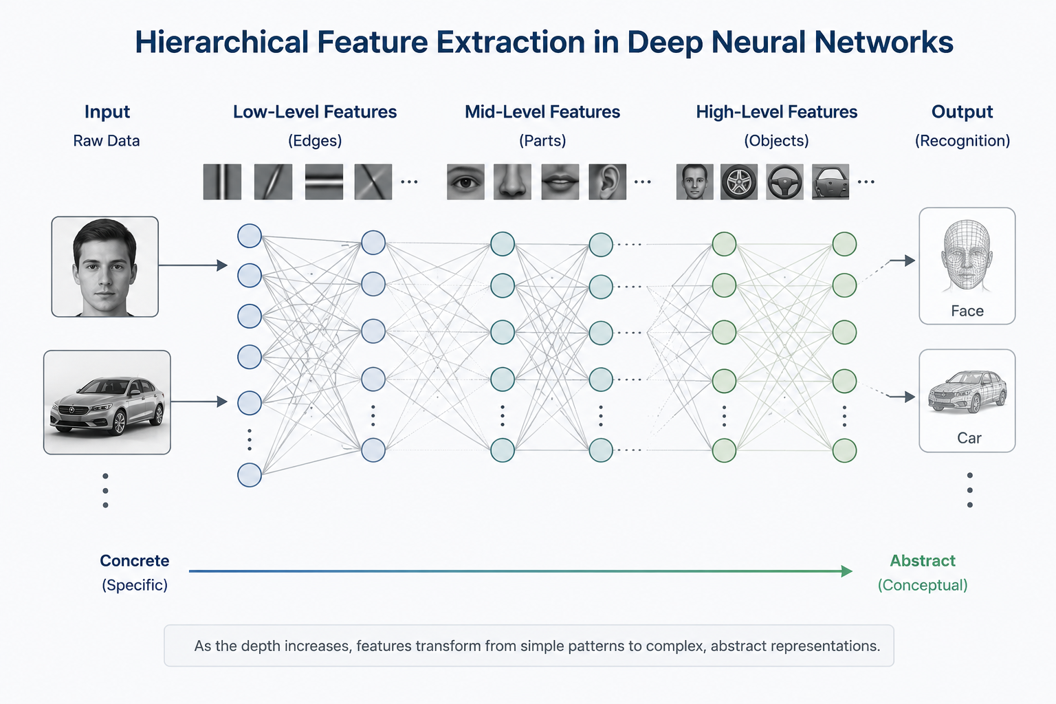
• Lower Layers - "Discovery of Points and Lines": These are the first layers data passes through. They detect the most basic visual elements, such as horizontal, vertical, or diagonal lines (edges), by checking the contrast between pixels.

• Mid Layers - "Assembly of Parts": These layers combine the lines found previously. Straight lines become curves, and intersecting lines form partial geometric shapes (parts) like wheel curves or square windows.

• Higher Layers - "Completion of Concepts": Parts are recombined to form concrete shapes like car bodies or grilles. Finally, the network understands that the collection of information is a single abstract concept: a "car".

1.2 Why 'Deep' Over 'Wide'? (The Economics of Efficiency)

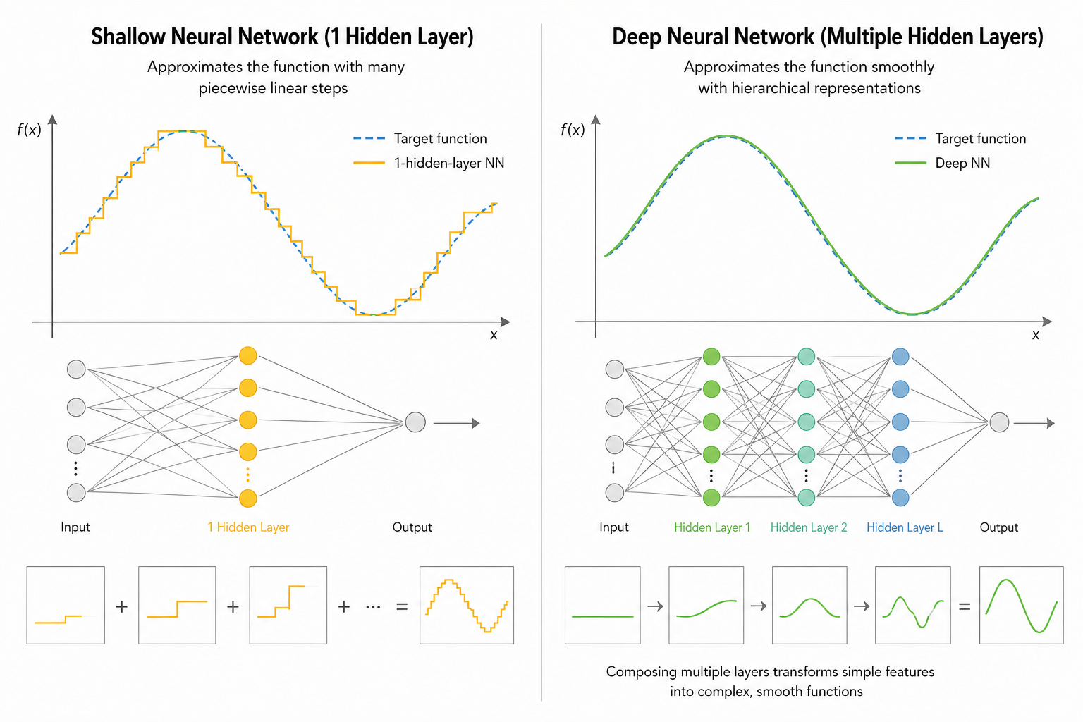
• Exponential Efficiency: While a "shallow and wide" network can theoretically represent any function (Universal Approximation Theorem), it requires an exponential increase in the number of nodes to handle complex data. Conversely, deep layers allow for the "reuse" of knowledge learned in previous layers, achieving superior performance with far fewer parameters.

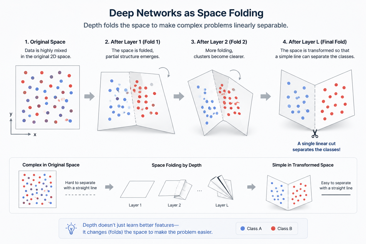
• Space Partitioning: As layers deepen, the network can "fold" and "twist" the input space more effectively, creating precise "hyperplanes" that cut through complexly tangled data.

2. Mathematical Proof: Universal Approximation Theorem

"If making a hidden layer infinitely wide can mimic any function, why can't we just use one wide layer?"

This is a sharp question often encountered when studying deep learning. According to the Universal Approximation Theorem, proven by Cybenko and others in 1989, a single hidden layer with an appropriate activation function can indeed approximate almost any continuous function we can imagine. However, there lies a massive trap of 'efficiency' that makes this practically impossible.

2.1 The Opportunity Cost of Depth vs. Width

Mathematical possibility does not always translate to engineering efficiency. The fatal limitations of a single-layer structure when expressing complex functions are as follows:

• Exponential Node Explosion: For a shallow network to match the complexity of a deep one, the number of nodes must grow exponentially ($2^n$). This leads to memory exhaustion and computational paralysis.

• Parameter Efficiency: Conversely, as layers deepen, functions become nested (Composition), allowing the model to reuse results from previous layers.

f(x) = \sigma(W_L \sigma(W_{L-1} ... \sigma(W_1 x + b_1) ...) + b_L)

Thanks to this hierarchical structure, deep networks express the same or even more complex functions elegantly with far fewer parameters. While a shallow layer tries to mimic the answer by 'patching pieces together,' a deep layer finds it by 'logical reasoning.'

2.2 Space Folding: Replicating the Brain's 3D Network

2.2.1 Solving Problems by Borrowing Dimensions

Consider two intertwined rings on a 2D plane; they cannot be separated without breaking. But if you move them into a 3D space, you can easily separate them by simply lifting one up. Just as our neurons intertwine in 3D to create thought, the 'depth' of deep learning physically twists and folds high-dimensional space. Each layer performs this 'dimensional magic':

• Space Transformation: At each layer, the network stretches and compresses the input space.

• Space Folding: Activation functions fold the space like paper.

\text{Input Space} \xrightarrow{\text{Layer 1}} \text{Folded Space} \xrightarrow{\text{Layer 2}} \text{Twisted Space}

As layers deepen, space is folded exponentially. Eventually, complex, tangled data is aligned into a simple, linear form. At the final output layer, a single straight line can elegantly solve a once-impossible problem.

3. The Necessity of Non-linear Activation Functions

The most important insight of this session is that 'depth without an activation function is merely a meaningless sequence of numbers.' Intelligence isn't born just by stacking layers. These small functions connecting the layers are the only keys to escaping the physical prison of 'linearity.'

3.1 The Curse of Linearity: Why 1,000 Layers Can Lead Nowhere

If you only repeat pure linear operations(y = Wx + b)without an activation function $\sigma$, what happens? Mathematically, the composition of linear transformations is just another linear transformation.

y = W_2(W_1 x)

Through the property of matrix multiplication, W_2 W_1 can be replaced by a single new matrix W_{new}. Even if you stack 1,000 layers, the model remains mathematically identical to a single-layer perceptron. The 'curved' boundaries needed for XOR problems are forever forbidden in a purely linear world.

3.2 The Magic of Non-linearity: Alchemy of Bending Space

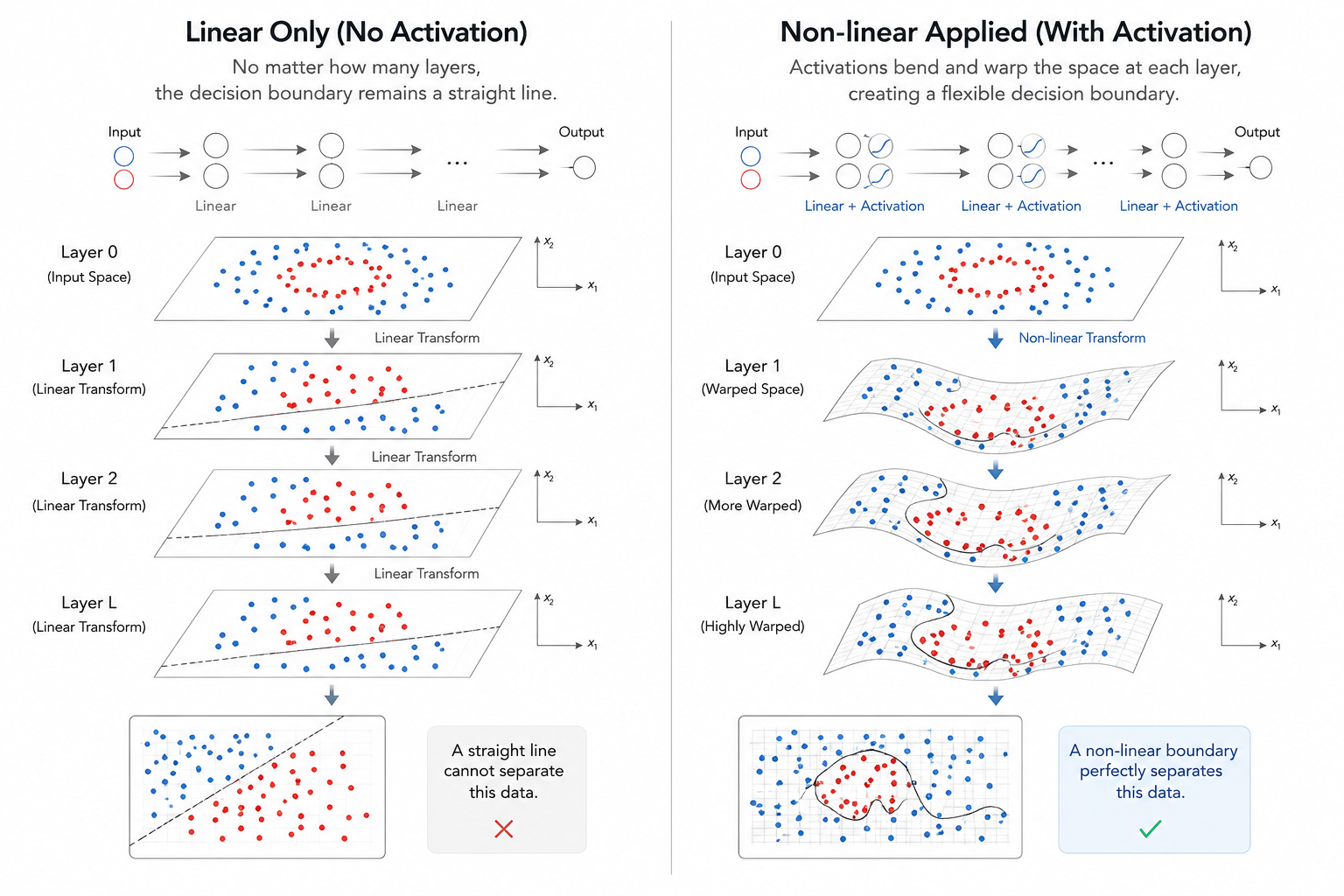
We intentionally inject Non-linearity into the output of each layer. This 'twist' allows the network to bend and fold space, performing high-level geometric operations to find the essence of data.

• Sigmoid: f(x) = \frac{1}{1+e^{-x}} (The Classic)

  Maps any input to a value between 0 and 1, allowing for probabilistic interpretation. However, it suffers from the 'Vanishing Gradient' problem, where learning stops as gradients converge to 0 for very large or small inputs.

• ReLU: f(x) = \max(0, x) (The Modern Standard)

  A simple structure that blocks signals below 0 and passes them if they are above 0. This simplicity maintains the 'vitality' of the signal even through complex derivatives, allowing modern deep learning to stack hundreds of layers.

• Tanh: f(x) = \frac{e^x - e^{-x}}{e^x + e^{-x}}

  Centers the output at 0 (-1 to 1), reducing bias for the next layer. It typically trains faster than Sigmoid and is still favored in specific architectures.

4. The Paradox of Depth: Trials That Come with Stature

Stacking layers isn't a guaranteed blessing. As models become more complex and deeper, serious side effects can occur where mathematical signals fail to deliver or the model loses sight of the data's essence.

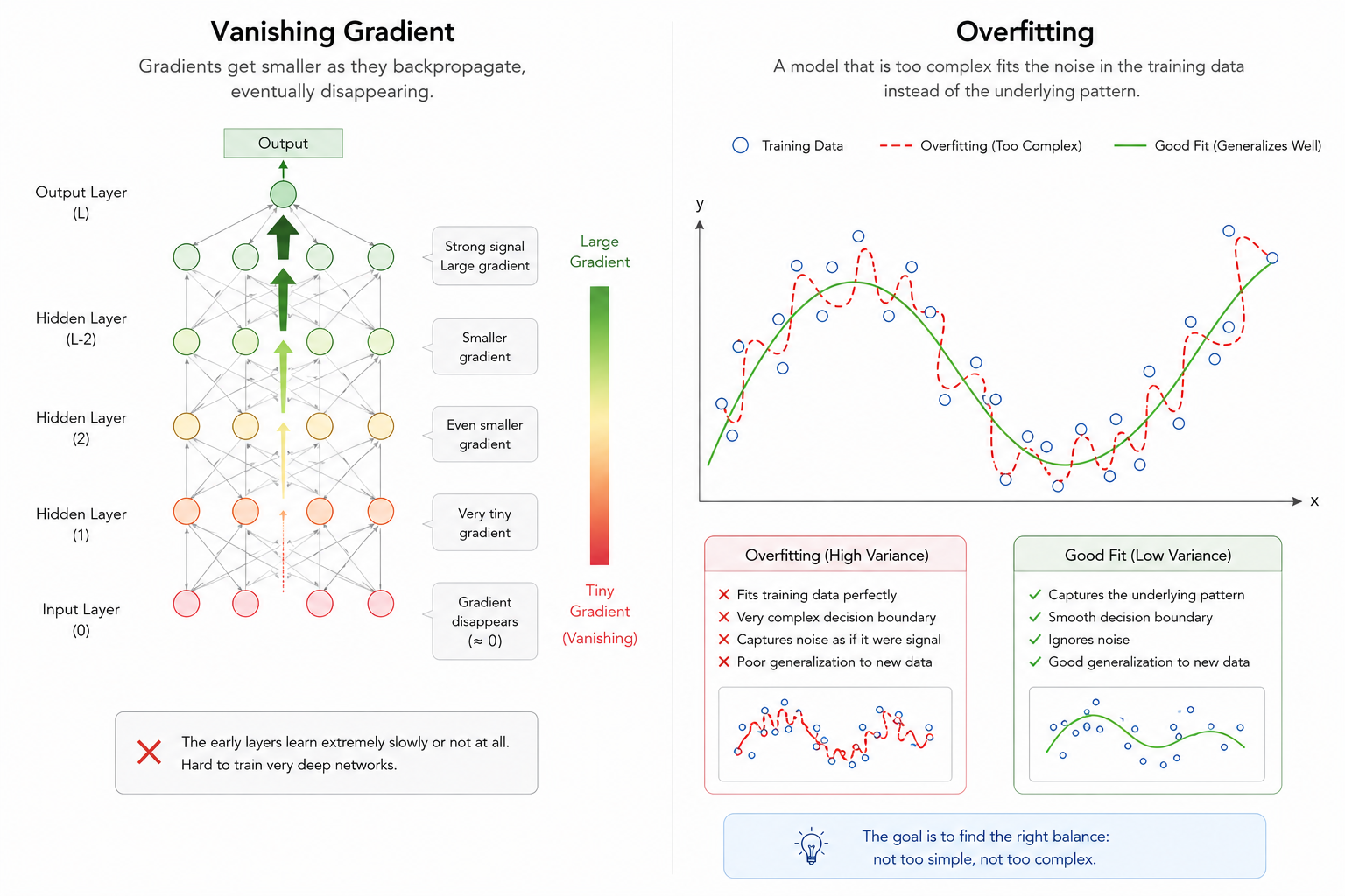
4.1 Vanishing Gradient: Signals Lost in the Abyss

Backpropagation updates weights by tracing errors from the output back to the input. During this, derivatives are continuously multiplied per the Chain Rule, which becomes the Achilles' heel of deep networks.

• Mathematical Decay: If an activation function (like Sigmoid) has derivatives less than 1 (e.g., < 0.25), these values multiply into something near zero as layers deepen.

• Stalled Updates: Front layers receive almost no error signal, causing learning to effectively stop.

4.2 Overfitting: Excessive Obsession with Data

Deepening a model increases its Expression Power (Capacity), but too much power can be toxic.

• Noise Learning: Deep models may learn the general features of data plus the meaningless noise or trivial patterns unique to that specific dataset.

• Generalization Failure: This results in high accuracy on training sets but poor performance on new, real-world data.

5. Conclusion: Depth is the Thickness of Logic

Today, we explored why AI had to become 'Deep.' Stacking layers is more than just increasing size; it is building the 'thickness of logic'—interpreting data from multiple angles, forming abstract concepts, and conquering the complexity of space.

However, as we’ve seen, depth alone isn't the answer. Signals weaken, and models become overly "obsessed" with specific data. In the next session, we will discuss the brilliant solutions to this 'curse of depth'—the revolution of activation functions and normalization—as we reach the finale of Season 1: Optimization.

Key Term Review

• Hierarchical Feature Extraction: Combining low-level features to form high-level abstract concepts.

• Universal Approximation Theorem: The mathematical basis that deep layers are more efficient at representing complex functions than shallow ones.

• Vanishing Gradient: The phenomenon where error signals disappear during backpropagation as the network deepens.

• Non-linearity: The essential mechanism that allows neural networks to draw complex curves and planes beyond simple straight lines.