Hello! I'm MitornAve.
In our last session, we witnessed the "Perceptron," the first cell of artificial intelligence, collapse in frustration against the wall of the XOR problem. It represented the complexity of a world that cannot be solved with a single straight line. But humanity did not stop there. We reasoned that if one line wasn't enough, we could overlap tens of thousands of them, allowing them to move organically to find the optimal path.
Today’s topic is the heart of modern AI: Backpropagation. Moving beyond the simple phrase "reducing error," let’s dive into the mathematical sophistication that allows these massive neural networks to actually "learn."
1. The Birth and Structure of Neural Networks: The Blueprint of the MLP
A perceptron, which can only produce a single output value, can only draw one straight line on a plane. Thus, while it could accurately bisect the simple logic of AND, OR, and NOT, it was stumped by XOR.
Decades after the perceptron was nearly forgotten, researchers including Geoffrey Hinton proposed a simple solution: "Just stack multiple perceptrons." In hindsight, this makes perfect sense. The human brain consists of countless neurons connected in complex ways; a single neuron cannot possibly simulate human thought.
To solve the XOR problem, we abandoned the single-layer structure and introduced the Multi-Layer Perceptron (MLP). We call this web-like structure of connected perceptrons an "Artificial Neural Network."
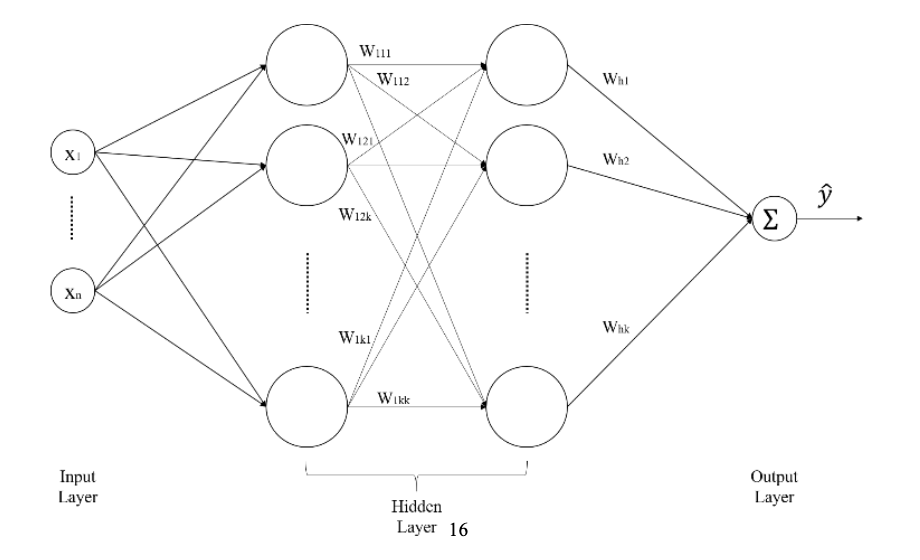
1) The 3-Tier Hierarchy of Neural Networks
Data flows through three primary layers:
Input Layer: This is where external data first enters the network. Pixel values from images or vector values from text are held in these nodes. No computation happens here; it simply passes data to the next layer.
Hidden Layer: The core of the network. It exists between the input and output layers, and because its processes aren't directly visible from the outside, it's called "Hidden." Here, countless weights ($w$) are calculated to extract complex patterns buried in the data. The "deeper" these layers go, the more high-dimensional features the network understands.
Output Layer: Where the final results emerge. In a classification problem, it might output the final judgment, such as "the probability that this data is a cat."
2) Activation Function: The Magic of Non-linearity
Simply stacking perceptrons doesn't mean you can draw curves. Mathematically, no matter how many linear operations (straight lines) you overlap, the result is still just one giant straight line.
This is where Activation Functions come in. Functions like Sigmoid, ReLU, and Tanh non-linearly "twist" the values calculated at each node. This "twist" allows the network to move beyond the limits of straight lines, forming curves or complex multi-dimensional planes (Hyperplanes) that elegantly solve the XOR problem.
2. The Essence of Learning: "Weights are the Only Key to Change"
Why do we obsess over weights (w) and biases (b) rather than other elements? It’s because they are the only "steering wheels" we can actually control in the massive function that is a neural network.
1) Fixed Environment, Unique Variable
The moment a deep learning model is designed and loaded into memory, many things become "constants":
Architecture: The number of layers, the number of nodes, and the choice of activation functions are already decided in the blueprint.
Data: The input images or text are also a given environment we cannot change.
However, a model immediately after initialization is like a blank slate. To make this "clumsy" model—which spits out random values when told to distinguish between dogs and cats—intelligent, we must adjust the weights, the connection strengths between nodes. It’s like a musician who cannot change the instrument (structure) but finely tunes the tension of the strings (weights) to create a beautiful melody.
2) Weights as the "Path of Intelligence"
Weights act as "importance coefficients" multiplied by the data signals flowing through the network:
Signal Extinction: If a weight converges to zero, that signal dies out and isn't passed to the next layer. The network has essentially decided that information is unnecessary for judgment.
Signal Amplification: Conversely, if a weight is large, that information survives strongly until the output stage, decisively influencing the final judgment.
Ultimately, learning is the process of optimization—precisely tightening and loosening millions of weights to minimize the Loss Function, which quantifies the distance between the correct answer and the predicted value.
3) Bias: The Power to Shift the Baseline
While weights adjust the "slope" of the signal, the bias (b) adjusts the "sensitivity," determining how easily a node is activated. Weights alone can only draw lines passing through the origin, but the addition of bias gives the network the "flexibility" to move anywhere in space to classify data.
3. The Mechanism of Backpropagation: The Revenge of Partial Derivatives and the Chain Rule
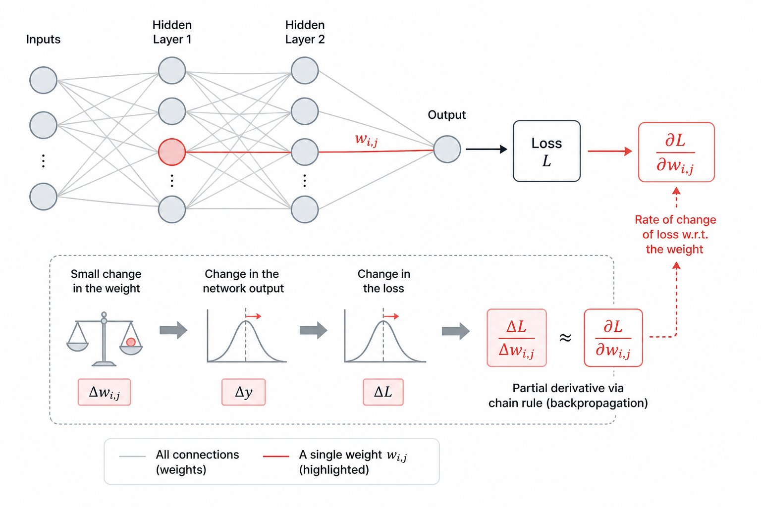
When the output layer says, "You’re wrong!", how much should we change a specific weight w_1 near the input layer? Changing them randomly involves too many possibilities. This is where mathematicians devised the Backward strategy.
1) Partial Derivative: Assigning Responsibility
How do we know how much a specific weight w_{ij} is "to blame" for the total error (E)? We use Partial Derivatives. (Yes, the scary math is back...)
A derivative measures how much something changes at a specific moment. A partial derivative is used when you want to calculate the change relative to only one specific attribute or target.
[Standard Derivative: The Speed of a Car]
The most common example is speed. When a car's position (y) changes over time (x), the derivative finds how fast the car is moving at a specific split second. Only one variable, "time," affects the position.
[Partial Derivative: Finding the Best Ramen Flavor]
Most things in the real world result from a mix of causes. Think of cooking delicious ramen (y). There are many variables: amount of water (x_1), heat intensity (x_2), and amount of soup base (x_3).
If we want to know how much the taste (y) changes when we only adjust the water (x_1) while keeping the heat and soup base constant, we use a partial derivative. It’s a declaration: "I will ignore everything else and measure the rate of change only for x_1."
In a neural network, a single output (prediction) involves millions of weights. If we simply differentiated the whole system, we couldn't tell which weight contributed to the answer and which one was the "culprit" creating the error.
By using partial derivatives, we focus on "only one weight (w_{ij})". Treating all other weights as constants, we calculate how much the final Loss fluctuates when that specific weight is changed slightly. We are asking: "Forget the other million connections for a second—how much is this specific line (w_{ij}) responsible for the total error (E)?"
2) Chain Rule: The Conduit of Error Energy
A neural network is a nested composite function:
y = f(g(h(x)))
It looks intimidating, but f, g, and h simply represent each layer. To find the derivative of the inner h(x), you must differentiate from the outside function and work your way in. This is the Chain Rule.
Error in Output Layer f: Calculate the Loss by comparing it to the answer.
Output Layer Weight Derivative: Calculate the influence the final weights had on the error.
Backpropagate to Hidden Layer: Use the derivative from the output layer to find the derivative of the layer before it.
Line-by-Line Tracking: Repeat this node-by-node and line-by-line until you reach the input layer.
\frac{\partial E}{\partial w_{ij}} = \underbrace{\frac{\partial E}{\partial out_j} \cdot \frac{\partial out_j}{\partial net_j}}_{\text{Node responsibility}} \cdot \underbrace{\frac{\partial net_j}{\partial w_{ij}}}_{\text{Weight contribution}}
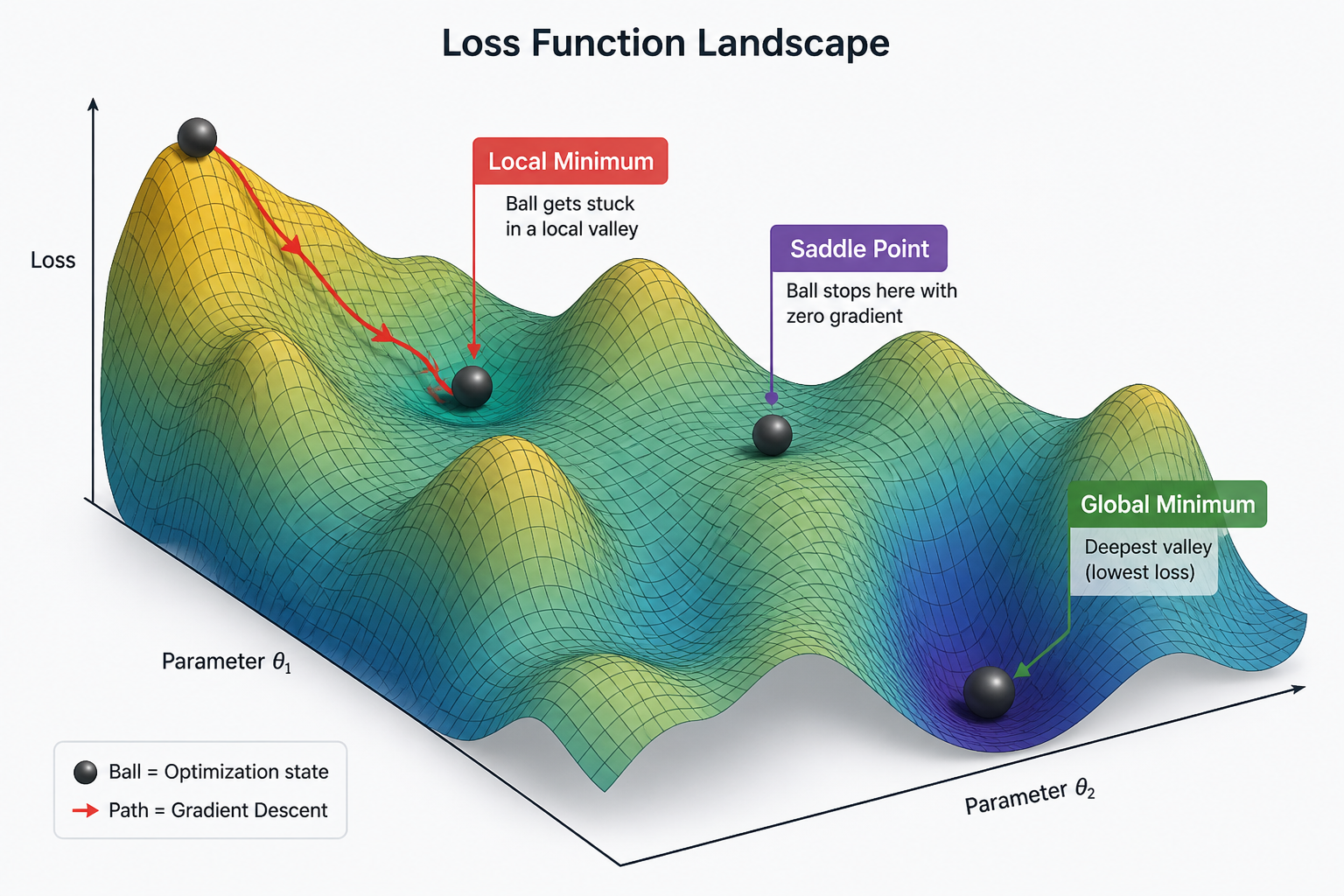
4. Gradient Descent: Toward the Valley of Truth
Now that we've identified the "responsibility" of each weight, we must move them. We are standing on a treacherous, foggy mountain range called "Error." Our goal is to reach the lowest point: the Global Minimum.
Backpropagation acts as our compass. Specifically, the Gradient (the rate of change of error relative to the weights) is our needle. The weight update formula is:
w \leftarrow w - \eta \frac{\partial E}{\partial w}
Positive Gradient (+): Increasing the weight increases the error, so we move in the negative (-) direction.
Negative Gradient (-): Increasing the weight decreases the error, so the two negatives make a plus (+), and we move in the positive direction.
The Learning Rate ($\eta$) determines our stride. If it's too large, we might skip over the valley floor and land on the opposite slope (Overshooting). If it's too small, it takes forever to descend, wasting computational resources.
However, this compass isn't perfect. We might fall into a Local Minimum—a small dip in the mountainside that isn't the true lowest point—or a Saddle Point, where the gradient is zero but it's not a minimum. These traps cause the algorithm to stall, thinking it has reached its goal when it hasn't.
5. Wrapping Up: The Beauty of Backward Intelligence
Today, we've explored the beautiful, grueling mathematical process by which a neural network corrects itself. From the multi-layer structures that warp space to find answers, to the chain rule of partial derivatives that points out the "culprit" weights. Without this backpropagation engine, ChatGPT and self-driving cars wouldn't exist.
Yet, even this "perfect" algorithm has a flaw. When layers get too deep, the shout of "You're wrong!" from the back can fade away before it ever reaches the front. This is the Vanishing Gradient problem.
Next time, we’ll see how humanity overcame this despair and opened the era of true "Deep" Learning.
Key Vocabulary Review
Hidden Layer: The heart of the network where abstract features are extracted.
Non-linear Activation Function: The device that turns a sum of lines into a curve to solve complex problems.
Partial Derivative: The mathematical investigation that identifies the fault of a single specific weight among millions.
Chain Rule: The logic that passes error energy backward through nested functions.
Learning Rate: The stride length when descending the mountain of error.